A Data Wrangling in R

In this part of our toolkit, we’re going to learn how to do the same things we did with Chapter 4 - Spatial Data Wrangling, but this time, we’ll use R code to handle our spatial data.

Getting Started

R is a great choice for starting in data science because it’s built for it. It’s not just a programming language, it is a whole system with tools and libraries made to help you think and work like a data scientist easily.

We assume a basic knowledge of R and coding languages for these toolkits. For most of the tutorials in this toolkit, you’ll need to have R and RStudio downloaded and installed on your system. You should be able to install packages, know how to find the address to a folder on your computer system, and have very basic familiarity with R.

Tutorials for R

If you are new to R, we recommend the following intro-level tutorials provided through installation guides. You can also refer to this R for Social Scientists tutorial developed by Data Carpentry for a refresher.

You can also visit the RStudio Education page to select a learning path tailored to your experience level (Beginners, Intermediates, Experts). They offer detailed instructions to learners at different stages of their R journey.

A.1 Environment Setup

Getting started with data analysis in R involves a few preliminary steps, including downloading datasets and setting up a working directory. This introduction will guide you through these essential steps to ensure a smooth start to your data analysis journey in R.

Download the Activity Datasets

Please download and unzip this file to get started: SDOHPlace-DataWrangling.zip

Setting Up the Working Directory

Setting up a working directory in R is crucial–any file paths you use in your code, like the names of files to read data from, will be treated at relative to your current working directly. You should set the working directory to any folder on your system where you plan to store your datasets and R scripts.

To set your working directory, use

setwd("/path/to/your/directory")

To see what your working directory is currently set to, use getwd().

A.1.0.1 Example: Local directory on Windows

You can use forward slashes for directory paths:

setwd("C:/Users/susan/RWork")

or you can use double backslashes:

setwd("C:\\Users\\susan\\RWork")

A.1.0.2 Example: Local directory on macOS or Linux

Use forward slashes:

setwd("/home/susan/RWork")

You can also use ~ as an abbreviation for your own home directory:

setwd("~/RWork")

A.1.0.3 Example: Posit Cloud

Posit Cloud is a web environment that allows you to create R projects online. In a Posit project, your working directory will already be set to your project. You can confirm this like so:

getwd()
[1] "/cloud/project"

Installing & Working with R Libraries

Before starting operations related to spatial data, we need to complete an environmental setup. This workshop requires several packages, which can be installed from CRAN:

• sf: simplifies spatial data manipulation
• tmap: streamlines thematic map creation
• dplyr: facilitates data manipulation
• tidygeocoder: converts addresses to coordinates easily

You only need to install packages once in an R environment. Use these commands to install the packages needed for this tutorial.

install.packages("sf")
install.packages("tmap")
install.packages("tidygeocoder")
install.packages("dplyr")

Installation Tip

For Mac users, check out https://github.com/r-spatial/sf for additional tips if you run into errors when installing the sf package. Using homebrew to install gdal usually fixes any remaining issues.

Now, loading the required libraries for further steps:

library(sf)
library(dplyr)
library(tmap)

A.2 Intro to Spatial Data

Spatial data analysis in R provides a robust framework for understanding geographical information, enabling users to explore, visualize, and model spatial relationships directly within their data. Through the integration of specialized packages like sf for spatial data manipulation, ggplot2 and tmap for advanced mapping, and tidygeocoder for geocoding, R becomes a powerful tool for geographic data science. This ecosystem allows researchers and analysts to uncover spatial patterns, analyze geographic trends, and produce detailed maps that convey complex information intuitively.

Load Spatial Data

We need to load the spatial data (shapefile). Remember, this type of data is actually comprised of multiple files. All need to be present in order to read correctly. Let’s use chicagotracts.shp for practice, which includes the census tracts boundary in Chicago.

First, we need to read the shapefile data from where you save it.

Chi_tracts = st_read("SDOHPlace-DataWrangling/chicagotracts.shp")

Your output will look something like:

## Reading layer `chicagotracts' from data source `./SDOHPlace-DataWrangling/chicagotracts.shp' using driver `ESRI Shapefile'
## Simple feature collection with 801 features and 9 fields
## Geometry type: POLYGON
## Dimension:     XY
## Bounding box:  xmin: -87.94025 ymin: 41.64429 xmax: -87.52366 ymax: 42.02392
## Geodetic CRS:  WGS 84

Always inspect data when loading in. Let’s look at a non-spatial view.

head(Chi_tracts)

## Simple feature collection with 6 features and 9 fields
## Geometry type: POLYGON
## Dimension:     XY
## Bounding box:  xmin: -87.68822 ymin: 41.72902 xmax: -87.62394 ymax: 41.87455
## Geodetic CRS:  WGS 84
##   commarea commarea_n countyfp10     geoid10 name10        namelsad10 notes statefp10 tractce10
## 1       44         44        031 17031842400   8424 Census Tract 8424  <NA>        17    842400
## 2       59         59        031 17031840300   8403 Census Tract 8403  <NA>        17    840300
## 3       34         34        031 17031841100   8411 Census Tract 8411  <NA>        17    841100
## 4       31         31        031 17031841200   8412 Census Tract 8412  <NA>        17    841200
## 5       32         32        031 17031839000   8390 Census Tract 8390  <NA>        17    839000
## 6       28         28        031 17031838200   8382 Census Tract 8382  <NA>        17    838200
##                         geometry
## 1 POLYGON ((-87.62405 41.7302...
## 2 POLYGON ((-87.68608 41.8229...
## 3 POLYGON ((-87.62935 41.8528...
## 4 POLYGON ((-87.68813 41.8556...
## 5 POLYGON ((-87.63312 41.8744...
## 6 POLYGON ((-87.66782 41.8741...

Check out the data structure of this file.

str(Chi_tracts)

## Classes 'sf' and 'data.frame':   801 obs. of  10 variables:
##  $ commarea  : chr  "44" "59" "34" "31" ...
##  $ commarea_n: num  44 59 34 31 32 28 65 53 76 77 ...
##  $ countyfp10: chr  "031" "031" "031" "031" ...
##  $ geoid10   : chr  "17031842400" "17031840300" "17031841100" "17031841200" ...
##  $ name10    : chr  "8424" "8403" "8411" "8412" ...
##  $ namelsad10: chr  "Census Tract 8424" "Census Tract 8403" "Census Tract 8411" "Census Tract 8412" ...
##  $ notes     : chr  NA NA NA NA ...
##  $ statefp10 : chr  "17" "17" "17" "17" ...
##  $ tractce10 : chr  "842400" "840300" "841100" "841200" ...
##  $ geometry  :sfc_POLYGON of length 801; first list element: List of 1
##   ..$ : num [1:243, 1:2] -87.6 -87.6 -87.6 -87.6 -87.6 ...
##   ..- attr(*, "class")= chr [1:3] "XY" "POLYGON" "sfg"
##  - attr(*, "sf_column")= chr "geometry"
##  - attr(*, "agr")= Factor w/ 3 levels "constant","aggregate",..: NA NA NA NA NA NA NA NA NA
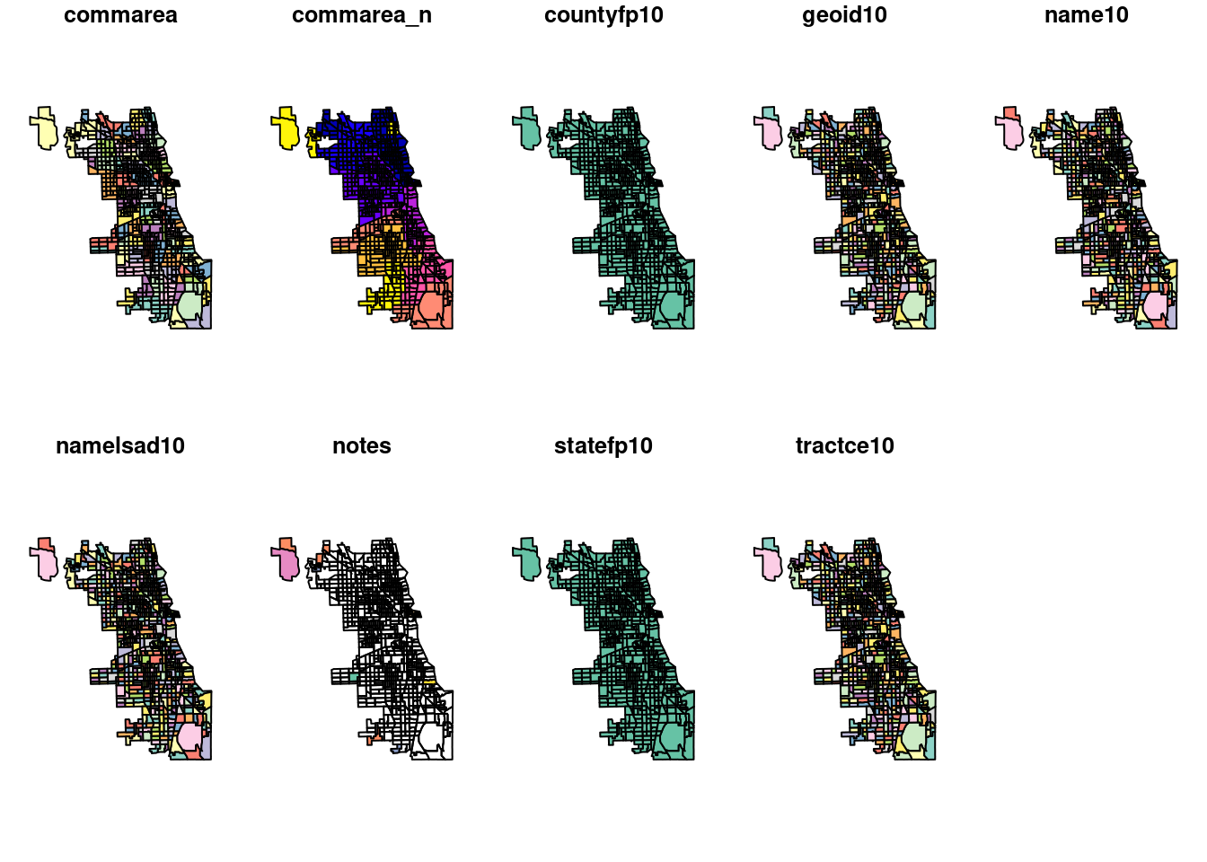
##   ..- attr(*, "names")= chr [1:9] "commarea" "commarea_n" "countyfp10" "geoid10" ...

The data is no longer a shapefile but an sf object, comprised of polygons. The plot() command in R help to quickly visualizes the geometric shapes of Chicago’s census tracts. The output includes multiple maps because the sf framework enables previews of each attribute in our spatial file.

plot(Chi_tracts)

A.2.1 Adding a Basemap

Then, we can use tmap, a mapping library, in interactive mode to add a basemap layer. It plots the spatial data from Chi_tracts, applies a minimal theme for clarity, and labels the map with a title, offering a straightforward visualization of the area’s census tracts.

We stylize the borders of the tract boundaries by making it transparent at 50% (which is equal to an alpha level of 0.5).

library(tmap)

tmap_mode("view")

## ℹ tmap mode set to "view".

tm_shape(Chi_tracts) + tm_borders(alpha=0.5) +
  tm_layout(title = "Census Tract Map of Chicago")

## 
## ── tmap v3 code detected ───────────────────────────────────────────────────────────────────────────────────────────────────
## [v3->v4] `tm_borders()`: use `fill_alpha` instead of `alpha`.[v3->v4] `tm_layout()`: use `tm_title()` instead of `tm_layout(title = )`

Still in the interactive mode (`view’), we can switch to a different basemap. Here we bring in a “Voyager” style map from Carto, a cartographic firm. We’ll make the borders less transparent by adjusting the alpha level.

tmap_mode("view")

## ℹ tmap mode set to "view".

tm_basemap("CartoDB.Voyager") + 
  tm_shape(Chi_tracts) + tm_borders(alpha=0.8, col = "gray40") +
  tm_layout(title = "Census Tract Map of Chicago")

## 
## ── tmap v3 code detected ───────────────────────────────────────────────────────────────────────────────────────────────────
## [v3->v4] `tm_borders()`: use `fill_alpha` instead of `alpha`.[v3->v4] `tm_layout()`: use `tm_title()` instead of `tm_layout(title = )`

Tip

For additional options, you can preview basemaps at the Leaflet Providers Demo. Some basemaps we recommend that work consistently are by:

• CartoDB (Carto)
• Open Street Map
• ESRI

Not all basemaps are available anymore, and some require keys that you’d need to add on your own.

A.3 Coordinate Reference Systems

For this exercise we will use chicagotracts.shp to explore how to change the projection of a spatial dataset in R. First, let’s check out the current coordinate reference system.

st_crs(Chi_tracts)

## Coordinate Reference System:
##   User input: WGS 84 
##   wkt:
## GEOGCRS["WGS 84",
##     DATUM["World Geodetic System 1984",
##         ELLIPSOID["WGS 84",6378137,298.257223563,
##             LENGTHUNIT["metre",1]]],
##     PRIMEM["Greenwich",0,
##         ANGLEUNIT["degree",0.0174532925199433]],
##     CS[ellipsoidal,2],
##         AXIS["latitude",north,
##             ORDER[1],
##             ANGLEUNIT["degree",0.0174532925199433]],
##         AXIS["longitude",east,
##             ORDER[2],
##             ANGLEUNIT["degree",0.0174532925199433]],
##     ID["EPSG",4326]]

We can use the st_transform function to transform CRS. When projecting a dataset of Illinois, the most appropriate NAD83 projection would be NAD83 UTM zone 16N. Chicago sits within the area best covered by NAD83 / Illinois East (ftUS) (EPSG:3435).

Chi_tracts.3435 <- st_transform(Chi_tracts, "EPSG:3435")
# Chi_tracts.3435 <- st_transform(Chi_tracts, 3435)
st_crs(Chi_tracts.3435)

## Coordinate Reference System:
##   User input: EPSG:3435 
##   wkt:
## PROJCRS["NAD83 / Illinois East (ftUS)",
##     BASEGEOGCRS["NAD83",
##         DATUM["North American Datum 1983",
##             ELLIPSOID["GRS 1980",6378137,298.257222101,
##                 LENGTHUNIT["metre",1]]],
##         PRIMEM["Greenwich",0,
##             ANGLEUNIT["degree",0.0174532925199433]],
##         ID["EPSG",4269]],
##     CONVERSION["SPCS83 Illinois East zone (US survey foot)",
##         METHOD["Transverse Mercator",
##             ID["EPSG",9807]],
##         PARAMETER["Latitude of natural origin",36.6666666666667,
##             ANGLEUNIT["degree",0.0174532925199433],
##             ID["EPSG",8801]],
##         PARAMETER["Longitude of natural origin",-88.3333333333333,
##             ANGLEUNIT["degree",0.0174532925199433],
##             ID["EPSG",8802]],
##         PARAMETER["Scale factor at natural origin",0.999975,
##             SCALEUNIT["unity",1],
##             ID["EPSG",8805]],
##         PARAMETER["False easting",984250,
##             LENGTHUNIT["US survey foot",0.304800609601219],
##             ID["EPSG",8806]],
##         PARAMETER["False northing",0,
##             LENGTHUNIT["US survey foot",0.304800609601219],
##             ID["EPSG",8807]]],
##     CS[Cartesian,2],
##         AXIS["easting (X)",east,
##             ORDER[1],
##             LENGTHUNIT["US survey foot",0.304800609601219]],
##         AXIS["northing (Y)",north,
##             ORDER[2],
##             LENGTHUNIT["US survey foot",0.304800609601219]],
##     USAGE[
##         SCOPE["Engineering survey, topographic mapping."],
##         AREA["United States (USA) - Illinois - counties of Boone; Champaign; Clark; Clay; Coles; Cook; Crawford; Cumberland; De Kalb; De Witt; Douglas; Du Page; Edgar; Edwards; Effingham; Fayette; Ford; Franklin; Gallatin; Grundy; Hamilton; Hardin; Iroquois; Jasper; Jefferson; Johnson; Kane; Kankakee; Kendall; La Salle; Lake; Lawrence; Livingston; Macon; Marion; Massac; McHenry; McLean; Moultrie; Piatt; Pope; Richland; Saline; Shelby; Vermilion; Wabash; Wayne; White; Will; Williamson."],
##         BBOX[37.06,-89.27,42.5,-87.02]],
##     ID["EPSG",3435]]

After change the projection, we can plot the map. We’ll switch to the static version of tmap, using the plot mode.

tmap_mode("plot")

## ℹ tmap mode set to "plot".

tm_shape(Chi_tracts.3435) + tm_borders(alpha=0.5) + 
  tm_layout(main.title ="EPSG:3435 (ft)",
             main.title.position = "center")

## 
## ── tmap v3 code detected ───────────────────────────────────────────────────────────────────────────────────────────────────
## [v3->v4] `tm_borders()`: use `fill_alpha` instead of `alpha`.[v3->v4] `tm_layout()`: use `tm_title()` instead of `tm_layout(main.title = )`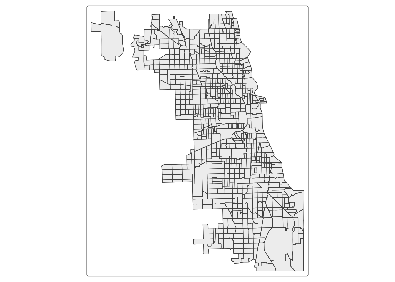

What if we had used the wrong EPSG code, referencing the wrong projection? Here we’ll transform and plot EPSG Code 3561, a coordinate reference system in Hawai’i.

Chi_tracts.3561 <- st_transform(Chi_tracts, "EPSG:3561")


tm_shape(Chi_tracts.3561) + tm_borders(alpha=0.5) + 
  tm_layout(main.title ="EPSG:3561 (ft)",
             main.title.position = "center")

## 

## ── tmap v3 code detected ───────────────────────────────────────────────────────────────────────────────────────────────────

## [v3->v4] `tm_borders()`: use `fill_alpha` instead of `alpha`.
## [v3->v4] `tm_layout()`: use `tm_title()` instead of `tm_layout(main.title = )`

It’s obviously not correct – the wrong CRS can cause a load of trouble. Make sure you specify carefully!

Refine Basic Map

Let’s take a deeper look at the cartographic mapping package, tmap. We approach mapping with one layer at a time. Always start with the object you want to map by calling it with the tm_shape function. Then, at least one descriptive/styling function follows. There are hundreds of variations and paramater specification.

Here we style the tracts with some semi-transparent borders.

library(tmap)

tm_shape(Chi_tracts) + tm_borders(alpha=0.5) 

## 

## ── tmap v3 code detected ───────────────────────────────────────────────────────────────────────────────────────────────────

## [v3->v4] `tm_borders()`: use `fill_alpha` instead of `alpha`.

Next we fill the tracts with a light gray, and adjust the color and transparency of borders. We also add a scale bar, positioning it to the left and having a thickness of 0.8 units, and turn off the frame.

tm_shape(Chi_tracts) + tm_fill(col = "gray90") + tm_borders(alpha=0.2, col = "gray10") +
  tm_scale_bar(position = ("bottom"), lwd = 0.8) +
  tm_layout(frame = F)

## 

## ── tmap v3 code detected ───────────────────────────────────────────────────────────────────────────────────────────────────

## [v3->v4] `tm_borders()`: use `fill_alpha` instead of `alpha`.
## ! `tm_scale_bar()` is deprecated. Please use `tm_scalebar()` instead.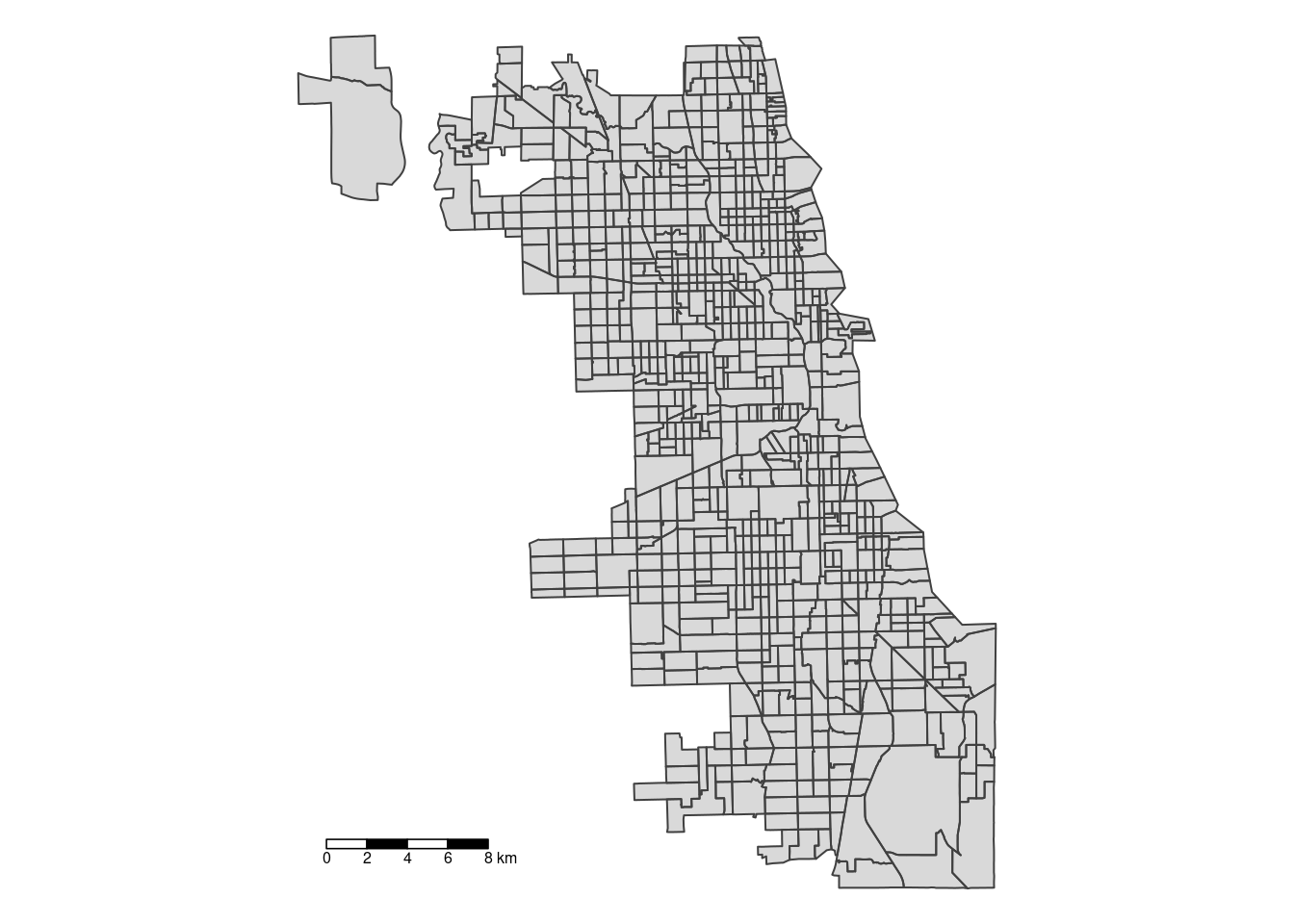

Check out https://rdrr.io/cran/tmap/man/tm_polygons.html for more ideas.

A.4 Converting to Spatial Data

A.4.1 Convert CSVs to Spatial Data

We are using the Affordable_Rental_Housing_Developments.csv in the dataset to show how to convert a csv Lat/Long data to points. First, we need to load the CSV data.

housing = read.csv("SDOHPlace-DataWrangling/Affordable_Rental_Housing_Developments.csv")

Then, we need to ensure that no column (intended to be used as a coordinate) is entirely empty or filled with NA values.

cleaned_housing <- na.omit(housing)

Inspect the data to confirm it’s doing what you expect it to be doing. What columns will you use to specify the coordinates? In this dataset, we have multiple coordinate options. We’ll use latitude and longitude, or rather, longitude as our X value, and latitude as our Y value. In the data, it’s specified as “Longitude” and “Latitude.”

head(cleaned_housing)

##   Community.Area.Name Community.Area.Number      Property.Type                   Property.Name                 Address
## 2         Rogers Park                     1             Senior              Morse Senior Apts.      6928 N. Wayne Ave.
## 3              Uptown                     3                ARO                      The Draper        5050 N. Broadway
## 4           Edgewater                    77             Senior                   Pomeroy Apts.    5650 N. Kenmore Ave.
## 5            Roseland                    49 Supportive Housing               Wentworth Commons 11045 S. Wentworth Ave.
## 6       Humboldt Park                    23        Multifamily            Nelson Mandela Apts.      607 N. Sawyer Ave.
## 7     Grand Boulevard                    38        Multifamily Legends South - Gwendolyn Place   4333 S. Michigan Ave.
##   Zip.Code Phone.Number               Management.Company Units X.Coordinate Y.Coordinate Latitude Longitude
## 2    60626 312-602-6207                 Morse Urban Dev.    44      1165844      1946059 42.00757 -87.66517
## 3    60640 312-818-1722                        Flats LLC    35      1167357      1933882 41.97413 -87.65996
## 4    60660 773-275-7820                  Habitat Company   198      1168181      1937918 41.98519 -87.65681
## 5    60628 773-568-7804          Mercy Housing Lakefront    50      1176951      1831516 41.69302 -87.62777
## 6    60624 773-227-6332                 Bickerdike Apts.     6      1154640      1903912 41.89215 -87.70753
## 7    60653 773-624-7676 Interstate Realty Management Co.    71      1177924      1876178 41.81555 -87.62286
##                                Location
## 2 (42.0075737709331, -87.6651711448293)
## 3 (41.9741295261027, -87.6599553011627)
## 4  (41.9851867755403, -87.656808676983)
## 5 (41.6930159120977, -87.6277673462214)
## 6 (41.8921534052465, -87.7075265659001)
## 7  (41.815550396096, -87.6228565224104)

Finally, we start to convert it to points. Be sure you use the CRS of the original coordinates recorded. In this case we weren’t sure what CRS that was, so we use EPSG:4326 to test.

points_housing <- st_as_sf(cleaned_housing, coords = c("Longitude", "Latitude"), crs = 4326)

View the resulting sf object with a basemap to confirm they are in the right place. Overlay them on top of the tract data, to confirm they are plotting correctly.

### First Layer
tm_shape(Chi_tracts) + tm_borders(lwd = 0.5) + 
  
  ### Second Layer
  tm_shape(points_housing) + tm_dots(size = 0.1 )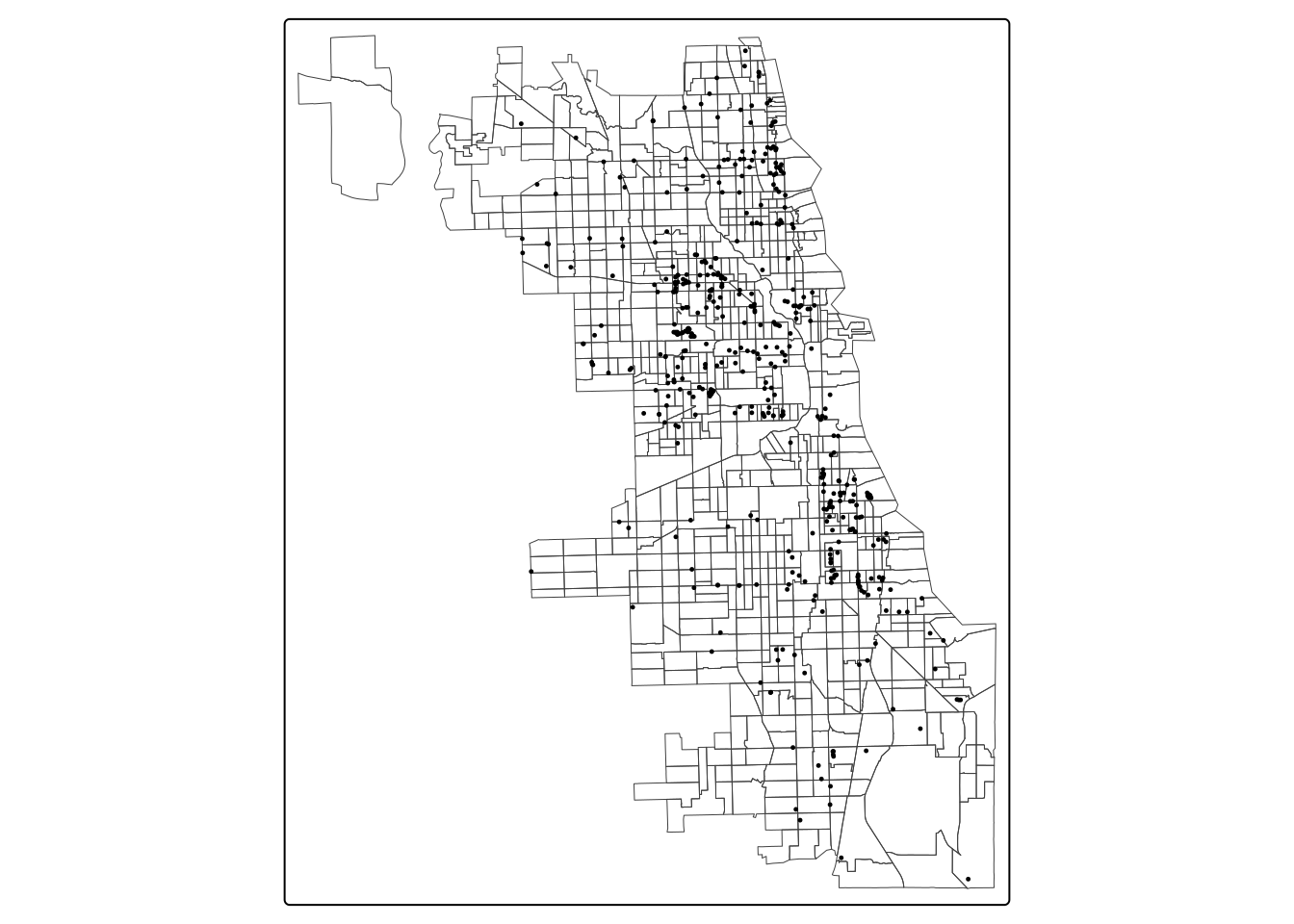

You can change the tmap_mode to “view” to add a basemap in an interactive setting, and then switch back to “plot” when complete. Because we’e plotting dots using tmap, we’ll use the tm_dots parameter for styling.

tmap_mode("view")

## ℹ tmap mode set to "view".

tm_shape(Chi_tracts) + tm_borders(lwd = 0.5) + 
  tm_shape(points_housing) + tm_dots(size = 0.01)

tmap_mode("plot")

## ℹ tmap mode set to "plot".

We’ll reproject to EPSG:3435, our system standard

housing.3435 <- st_transform(points_housing, "EPSG:3435")

A.4.1.1 Write Spatial Data

Finally, we can save our points as a spatial dataset. Use ‘st_write’ to write your spatial object in R to a data format of your choice. Here, we’ll write to a geojson file.

st_write(housing.3435, "housing.geojson", driver = "GeoJSON")

You could also save as a “housing.shapefile” to get a shapefile format, however you’ll get an error noting that some column names are too long and must be shortened. Shapefiles have a limit of 10 characters for field names.

st_write(housing.3435, "housing.shp", driver = "ESRI Shapefile")

The file may still write, but the column names that were too long may be shortened automatically.

To change column or field names in R objects, there are dozens of options. Try searching and “Googling” different search terms to identify solutions on your own.

A.4.2 Geocode Addresses

Here, we will use chicago_methadone_nogeometry.csv for practice, which includes methadone centers in Chicago (center names and addresses). First we load the tidygeocoder library to get our geocoding done.

library(tidygeocoder)

Let’s read in and inspect data for methadone maintenance providers. Note, these addresses were made available by SAMHSA, and are known as publicly available information. An additional analysis could call each service to check on access to medication during COVID in September 2020, and the list would be updated further.

methadoneClinics <- read.csv("SDOHPlace-DataWrangling/chicago_methadone_nogeometry.csv")

head(methadoneClinics)

##   X                                                         Name                 Address    City State   Zip
## 1 1                Chicago Treatment and Counseling Center, Inc. 4453 North Broadway st. Chicago    IL 60640
## 2 2                      Sundace Methadone Treatment Center, LLC 4545 North Broadway St. Chicago    IL 60640
## 3 3 Soft Landing Interventions/DBA Symetria Recovery of Lakeview    3934 N. Lincoln Ave. Chicago    IL 60613
## 4 4                                        PDSSC - Chicago, Inc.     2260 N. Elston Ave. Chicago    IL 60614
## 5 5                          Center for Addictive Problems, Inc.        609 N. Wells St. Chicago    IL 60654
## 6 6                                Family Guidance Centers, Inc.     310 W. Chicago Ave. Chicago    IL 60654

Let’s geocode one address first, just to make sure our system is working. We’ll use the “osm” method to use the OpenStreetMap geocoder.

sample <- geo("2260 N. Elston Ave. Chicago, IL", lat = latitude, long = longitude, method = 'osm')

## Passing 1 address to the Nominatim single address geocoder

## Query completed in: 1.8 seconds

head(sample)

## # A tibble: 1 × 3
##   address                         latitude longitude
##   <chr>                              <dbl>     <dbl>
## 1 2260 N. Elston Ave. Chicago, IL     41.9     -87.7

As we prepare for geocoding, check out the structure of the dataset. The data should be a character to be read properly.

str(methadoneClinics)

## 'data.frame':    27 obs. of  6 variables:
##  $ X      : int  1 2 3 4 5 6 7 8 9 10 ...
##  $ Name   : chr  "Chicago Treatment and Counseling Center, Inc." "Sundace Methadone Treatment Center, LLC" "Soft Landing Interventions/DBA Symetria Recovery of Lakeview" "PDSSC - Chicago, Inc." ...
##  $ Address: chr  "4453 North Broadway st." "4545 North Broadway St." "3934 N. Lincoln Ave." "2260 N. Elston Ave." ...
##  $ City   : chr  "Chicago" "Chicago" "Chicago" "Chicago" ...
##  $ State  : chr  "IL" "IL" "IL" "IL" ...
##  $ Zip    : int  60640 60640 60613 60614 60654 60654 60651 60607 60607 60616 ...

We need to clean the data a bit. We’ll add a new column for a full address, as required by the geocoding service. When you use a geocoding service, be sure to read the documentation and understand how the data needs to be formatted for input.

methadoneClinics$fullAdd <- paste(as.character(methadoneClinics$Address), 
                                  as.character(methadoneClinics$City),
                                  as.character(methadoneClinics$State), 
                                  as.character(methadoneClinics$Zip))

We’re ready to go! Batch geocode with one function, and inspect:

geoCodedClinics <-  geocode(methadoneClinics,
address = 'fullAdd', lat = latitude, long = longitude, method="osm")

## Passing 27 addresses to the Nominatim single address geocoder

## Query completed in: 33.4 seconds

head(geoCodedClinics)

## # A tibble: 6 × 9
##       X Name                                                         Address    City  State   Zip fullAdd latitude longitude
##   <int> <chr>                                                        <chr>      <chr> <chr> <int> <chr>      <dbl>     <dbl>
## 1     1 Chicago Treatment and Counseling Center, Inc.                4453 Nort… Chic… IL    60640 4453 N…     42.0     -87.7
## 2     2 Sundace Methadone Treatment Center, LLC                      4545 Nort… Chic… IL    60640 4545 N…     42.0     -87.7
## 3     3 Soft Landing Interventions/DBA Symetria Recovery of Lakeview 3934 N. L… Chic… IL    60613 3934 N…     42.0     -87.7
## 4     4 PDSSC - Chicago, Inc.                                        2260 N. E… Chic… IL    60614 2260 N…     41.9     -87.7
## 5     5 Center for Addictive Problems, Inc.                          609 N. We… Chic… IL    60654 609 N.…     41.9     -87.6
## 6     6 Family Guidance Centers, Inc.                                310 W. Ch… Chic… IL    60654 310 W.…     41.9     -87.6

In some cases you may find that an address does not geocode correctly. You can inspect further. This could involve a quick check for spelling issues or searching the address and pulling the lat/long using Google Maps and inputting manually. Or, if we are concerned it’s a human or unknown error, we could omit. For this exercise we’ll just omit the two clinics that didn’t geocode correctly.

geoCodedClinics2 <- na.omit(geoCodedClinics)

A.5 Convert to Spatial Data

This is not spatial data yet! To convert a static file to spatial data, we use the powerful st_as_sf function from sf. Indicate the x,y parameters (=longitude, latitude) and the coordinate reference system used. Our geocoding service used the standard EPSG:4326, so we input that here.

methadoneSf <- st_as_sf(geoCodedClinics2, 
                        coords = c( "longitude", "latitude"),
                        crs = 4326)

Basic Map of Points

For a really simple map of points – to ensure they were geocoded and converted to spatial data correctly, we use tmap. We’ll use the interactive version to view.

tmap_mode("view")

tm_shape(methadoneSf) + tm_dots() 

If your points didn’t plot correctly:

• Did you flip the longitude/latitude values?
• Did you input the correct CRS?

Those two issues are the most common errors.

A.6 Merge Data sets

Reshape Data

Here, we are trying to use the COVID-19_Cases__Tests__and_Deaths_by_ZIP_Code.csv dataset to practice how to convert long data to a wide data format.

We subset to the first two columns, and the sixth column. That gives us the zip code, the reporting week, and cumulative cases of Covid-19. Choose whatever subset function you prefer best!

covid = read.csv("SDOHPlace-DataWrangling/COVID-19_Cases__Tests__and_Deaths_by_ZIP_Code.csv")

covid_clean = covid[,c(1:2, 6)]

head(covid_clean) 

##   ZIP.Code Week.Number Cases...Cumulative
## 1    60603          39                 13
## 2    60604          39                 31
## 3    60611          16                 72
## 4    60611          15                 64
## 5    60615          11                 NA
## 6    60603          10                 NA

Now, we want each zip code to be a unique row, with cases by week as a columns because we are trying to create a wide data set with the cumulative cases for each week for each zip code. Enter the code and you will see the new wide data format.

covid_wide <- reshape(covid_clean, direction = "wide",
                      idvar = "ZIP.Code", timevar = "Week.Number") 
head(covid_wide)

##    ZIP.Code Cases...Cumulative.39 Cases...Cumulative.16 Cases...Cumulative.15 Cases...Cumulative.11 Cases...Cumulative.10
## 1     60603                    13                    NA                    NA                    NA                    NA
## 2     60604                    31                    NA                    NA                    NA                    NA
## 3     60611                   458                    72                    64                    NA                    NA
## 5     60615                   644                   171                   132                    NA                    NA
## 31    60605                   391                    93                    65                    NA                    NA
## 32  Unknown                   240                    23                    18                    NA                    NA
##    Cases...Cumulative.12 Cases...Cumulative.13 Cases...Cumulative.14 Cases...Cumulative.34 Cases...Cumulative.17
## 1                     NA                    NA                    NA                    11                    NA
## 2                     NA                    NA                    NA                    29                     6
## 3                     16                    41                    57                   352                    80
## 5                     26                    57                    99                   567                   215
## 31                    23                    39                    52                   325                   118
## 32                    NA                    NA                     9                   162                    33
##    Cases...Cumulative.18 Cases...Cumulative.19 Cases...Cumulative.20 Cases...Cumulative.31 Cases...Cumulative.22
## 1                     NA                    NA                     5                     9                     6
## 2                     11                    14                    17                    25                    22
## 3                     92                    99                   114                   286                   139
## 5                    243                   274                   302                   526                   353
## 31                   135                   149                   155                   291                   187
## 32                    53                    62                    69                   127                    97
##    Cases...Cumulative.23 Cases...Cumulative.24 Cases...Cumulative.25 Cases...Cumulative.28 Cases...Cumulative.29
## 1                      6                     6                     6                     6                     8
## 2                     23                    24                    24                    25                    25
## 3                    148                   152                   163                   223                   240
## 5                    364                   376                   388                   444                   482
## 31                   194                   198                   215                   247                   263
## 32                   102                   106                   112                   120                   124
##    Cases...Cumulative.30 Cases...Cumulative.32 Cases...Cumulative.33 Cases...Cumulative.26 Cases...Cumulative.27
## 1                      9                    10                    11                     6                     6
## 2                     25                    25                    25                    25                    25
## 3                    264                   305                   333                   175                   196
## 5                    506                   539                   556                   401                   418
## 31                   277                   304                   312                   229                   235
## 32                   126                   132                   142                   113                   116
##    Cases...Cumulative.36 Cases...Cumulative.38 Cases...Cumulative.21 Cases...Cumulative.35 Cases...Cumulative.37
## 1                     11                    13                     6                    11                    13
## 2                     31                    31                    20                    30                    31
## 3                    391                   435                   124                   371                   411
## 5                    606                   629                   332                   588                   613
## 31                   354                   379                   169                   333                   364
## 32                   186                   216                    92                   178                   201
##    Cases...Cumulative.40
## 1                     14
## 2                     31
## 3                    478
## 5                    651
## 31                   399
## 32                   288

Join by Attribute

Here, we’ll merge data sets with a common variable in R. Merging the cumulative case data set you created in the last section to zip code spatial data (ChiZipMaster1.geojson) will allow you to map the case data. You’ll be merging the case data and spatial data using the zip codes field of each dataset.

We’ve cleaned our covid case data already, but not all values under the zip code column are valid. There is a row has a value of “unknown”, so let’s remove that.

covid_wide_clean <- covid_wide %>%
  filter(ZIP.Code != "unknown" & !is.na(ZIP.Code))

Then, we need to load the zip code data.

zipcode <- st_read("SDOHPlace-DataWrangling/ChiZipMaster1.geojson")

Your output will look something like:

Reading layer `ChiZipMaster1' from data source `./SDOHPlace-DataWrangling/ChiZipMaster1.geojson' using driver `GeoJSON'
Simple feature collection with 59 features and 30 fields
Geometry type: MULTIPOLYGON
Dimension:     XY
Bounding box:  xmin: -87.94011 ymin: 41.64454 xmax: -87.52414 ymax: 42.02304
Geodetic CRS:  WGS 84

Now, the two datasets are ready to join together by the zip code. Make sure to check they have been joined successully.

We call the these joined datasets Chi_Zipsf, to denote a final zip code master dataset.

Chi_Zipsf <- zipcode %>%
  left_join(covid_wide_clean, by = c("zip" = "ZIP.Code"))

We’ll reproject to EPSG:3435, the standard used in our study area.

Chi_Zipsf.3435 <- st_transform(Chi_Zipsf, 3435)

Join by Location

We’ll create a spatial join with the housing and zip code data we’ve brought in.

In this example, we want to join zip-level data to the Rental Housing Developments, so we can identify which zips they are within.

First, let’s try “sticking” all the zip code data to the housing points, essentially intersecting zip codes with housing developments.

To do this, both datasets will need to be in the same CRS. We have already standardized both using EPSG:3435.

Housing.f <- st_join(housing.3435, Chi_Zipsf.3435, join = st_intersects)

Don’t forget to inspect the data.

head(Housing.f)

## Simple feature collection with 6 features and 73 fields
## Geometry type: POINT
## Dimension:     XY
## Bounding box:  xmin: 1154639 ymin: 1831516 xmax: 1177923 ymax: 1946059
## Projected CRS: NAD83 / Illinois East (ftUS)
##   Community.Area.Name Community.Area.Number      Property.Type                   Property.Name                 Address
## 2         Rogers Park                     1             Senior              Morse Senior Apts.      6928 N. Wayne Ave.
## 3              Uptown                     3                ARO                      The Draper        5050 N. Broadway
## 4           Edgewater                    77             Senior                   Pomeroy Apts.    5650 N. Kenmore Ave.
## 5            Roseland                    49 Supportive Housing               Wentworth Commons 11045 S. Wentworth Ave.
## 6       Humboldt Park                    23        Multifamily            Nelson Mandela Apts.      607 N. Sawyer Ave.
## 7     Grand Boulevard                    38        Multifamily Legends South - Gwendolyn Place   4333 S. Michigan Ave.
##   Zip.Code Phone.Number               Management.Company Units X.Coordinate Y.Coordinate
## 2    60626 312-602-6207                 Morse Urban Dev.    44      1165844      1946059
## 3    60640 312-818-1722                        Flats LLC    35      1167357      1933882
## 4    60660 773-275-7820                  Habitat Company   198      1168181      1937918
## 5    60628 773-568-7804          Mercy Housing Lakefront    50      1176951      1831516
## 6    60624 773-227-6332                 Bickerdike Apts.     6      1154640      1903912
## 7    60653 773-624-7676 Interstate Realty Management Co.    71      1177924      1876178
##                                Location   zip SHAPE_AREA SHAPE_LEN Case.Rate...Cumulative year totPopE whiteP blackP amIndP
## 2 (42.0075737709331, -87.6651711448293) 60626   49170579  33983.91                 2911.7 2018   49730  59.20  25.27   0.10
## 3 (41.9741295261027, -87.6599553011627) 60640   77305246  48985.87                 1843.2 2018   69715  64.27  16.96   0.50
## 4  (41.9851867755403, -87.656808676983) 60660   37984389  27307.81                 1778.4 2018   43242  65.53  14.35   0.29
## 5 (41.6930159120977, -87.6277673462214) 60628  345241692  83748.99                 2562.8 2018   66724   4.40  93.75   0.07
## 6 (41.8921534052465, -87.7075265659001) 60624   99418123  40394.41                 3434.9 2018   36158   3.69  90.85   0.04
## 7  (41.815550396096, -87.6228565224104) 60653   67759828  34316.36                 2430.3 2018   31972   5.22  91.00   0.29
##   asianP pacIsP otherP hispP noHSP age0_4 age5_14 age15_19 age20_24 age15_44 age45_49 age50_54 age55_59 age60_64 ageOv65
## 2   5.89   0.01   9.53 20.62 11.82   2553    4765     2937     5056    25875     3295     3051     2713     2447    5031
## 3  11.03   0.03   7.21 14.26 10.31   3256    5183     1721     4535    35010     4966     4821     4142     3350    8987
## 4  13.03   0.02   6.77 17.87 10.54   1891    2448     2469     3289    22266     2821     2962     2513     2600    5741
## 5   0.18   0.02   1.58  3.44 14.84   4153    8578     4461     5226    25566     4574     4189     4764     3628   11272
## 6   0.31   0.08   5.03  5.30 26.14   3276    6034     2693     2935    15257     1913     2200     2032     1524    3922
## 7   1.34   0.00   2.15  2.16 14.92   2632    4990     1975     1811    12889     2200     1486     1883     1770    4122
##   ageOv18 age18_64 a15_24P und45P ovr65P disbP Cases...Cumulative.39 Cases...Cumulative.16 Cases...Cumulative.15
## 2   41428    36397   16.07  66.75  10.12  10.8                  1448                   301                   166
## 3   60170    51183    8.97  62.32  12.89  11.7                  1285                   319                   175
## 4   38197    32456   13.32  61.53  13.28  12.3                   769                   182                   115
## 5   51211    39939   14.52  57.40  16.89  15.9                  1710                   413                   317
## 6   25134    21212   15.57  67.94  10.85  18.6                  1242                   334                   242
## 7   23060    18938   11.84  64.15  12.89  17.8                   777                   238                   176
##   Cases...Cumulative.11 Cases...Cumulative.10 Cases...Cumulative.12 Cases...Cumulative.13 Cases...Cumulative.14
## 2                    NA                    NA                    17                    40                    83
## 3                    NA                    NA                    22                    57                   101
## 4                    NA                    NA                    16                    35                    63
## 5                    NA                    NA                    27                   123                   242
## 6                    NA                    NA                    19                    76                   166
## 7                    NA                    NA                    21                    67                   114
##   Cases...Cumulative.34 Cases...Cumulative.17 Cases...Cumulative.18 Cases...Cumulative.19 Cases...Cumulative.20
## 2                  1352                   501                   629                   735                   831
## 3                  1130                   467                   567                   633                   696
## 4                   637                   224                   274                   314                   342
## 5                  1547                   647                   758                   858                   932
## 6                  1124                   417                   510                   598                   671
## 7                   716                   286                   324                   376                   425
##   Cases...Cumulative.31 Cases...Cumulative.22 Cases...Cumulative.23 Cases...Cumulative.24 Cases...Cumulative.25
## 2                  1279                  1006                  1074                  1103                  1118
## 3                  1051                   791                   813                   843                   862
## 4                   574                   410                   432                   442                   464
## 5                  1408                  1057                  1077                  1104                  1135
## 6                  1040                   833                   858                   871                   893
## 7                   670                   496                   514                   528                   541
##   Cases...Cumulative.28 Cases...Cumulative.29 Cases...Cumulative.30 Cases...Cumulative.32 Cases...Cumulative.33
## 2                  1208                  1238                  1262                  1296                  1322
## 3                   954                   987                  1016                  1081                  1103
## 4                   516                   534                   557                   587                   618
## 5                  1260                  1309                  1366                  1462                  1497
## 6                   974                   997                  1020                  1058                  1090
## 7                   601                   622                   648                   689                   702
##   Cases...Cumulative.26 Cases...Cumulative.27 Cases...Cumulative.36 Cases...Cumulative.38 Cases...Cumulative.21
## 2                  1142                  1169                  1384                  1425                   913
## 3                   880                   913                  1200                  1250                   756
## 4                   482                   492                   685                   736                   379
## 5                  1166                  1202                  1629                  1683                  1003
## 6                   915                   942                  1177                  1217                   778
## 7                   562                   578                   743                   762                   474
##   Cases...Cumulative.35 Cases...Cumulative.37 Cases...Cumulative.40                geometry
## 2                  1362                  1407                  1468 POINT (1165843 1946059)
## 3                  1167                  1218                  1309 POINT (1167356 1933883)
## 4                   666                   702                   791 POINT (1168180 1937919)
## 5                  1579                  1656                  1742 POINT (1176951 1831516)
## 6                  1146                  1190                  1259 POINT (1154639 1903912)
## 7                   727                   753                   789 POINT (1177923 1876178)

We could also flip things around, and try to count how many developments intersect each zip code. We can use lengths() to find out how many items are present in a vector.

Chi_Zipsf.3435$TotHousing <- lengths(st_intersects(Chi_Zipsf.3435, housing.3435))

head(Chi_Zipsf.3435)

## Simple feature collection with 6 features and 62 fields
## Geometry type: MULTIPOLYGON
## Dimension:     XY
## Bounding box:  xmin: 1161881 ymin: 1818580 xmax: 1190986 ymax: 1902960
## Projected CRS: NAD83 / Illinois East (ftUS)
##     zip SHAPE_AREA SHAPE_LEN Case.Rate...Cumulative year totPopE whiteP blackP amIndP asianP pacIsP otherP hispP noHSP
## 1 60607   64664294  39143.64                 2504.1 2018   29591  58.17  14.51   0.13  22.58   0.10   4.51  8.30  3.94
## 2 60661    9357756  13132.57                 1531.3 2018    9926  57.29   3.60   0.00  35.79   0.00   3.31  6.45  0.58
## 3 60606    6766411  12040.44                 2289.6 2018    3101  72.75   2.35   0.00  18.09   0.00   6.80  6.29  0.73
## 4 60615   66565455  38321.31                 1549.5 2018   41563  30.10  55.22   0.35   8.09   0.00   6.23  6.19  6.05
## 5 60643  207706233  75254.73                 2422.3 2018   49870  22.24  73.53   0.14   0.36   0.02   3.70  3.31  8.48
## 6 60621  104746821  42299.92                 2647.9 2018   29042   2.58  94.77   0.28   0.26   0.00   2.12  3.65 22.16
##   age0_4 age5_14 age15_19 age20_24 age15_44 age45_49 age50_54 age55_59 age60_64 ageOv65 ageOv18 age18_64 a15_24P und45P
## 1   1660    1392     2351     4588    20860     1392      859     1122      702    1604   26241    24637   23.45  80.81
## 2    447     150      160     1032     7897      417      322      301      175     217    9243     9026   12.01  85.57
## 3     57      44        0      139     1863      213      153      168      172     431    3000     2569    4.48  63.33
## 4   2006    3512     2088     5317    21182     2293     2193     2095     2260    6022   34890    28868   17.82  64.24
## 5   3134    5603     3385     3277    17324     3225     4061     4044     3326    9153   38788    29635   13.36  52.26
## 6   2504    4102     1893     2260    11246     1317     2146     1927     1872    3928   21232    17304   14.30  61.47
##   ovr65P disbP Cases...Cumulative.39 Cases...Cumulative.16 Cases...Cumulative.15 Cases...Cumulative.11
## 1   5.42   6.1                   741                   320                   283                    NA
## 2   2.19   2.3                   152                    20                    17                    NA
## 3  13.90   1.9                    71                    13                     7                    NA
## 4  14.49  12.0                   644                   171                   132                    NA
## 5  18.35  13.8                  1208                   344                   284                    NA
## 6  13.53  20.1                   769                   219                   143                    NA
##   Cases...Cumulative.10 Cases...Cumulative.12 Cases...Cumulative.13 Cases...Cumulative.14 Cases...Cumulative.34
## 1                    NA                    17                    46                    79                   623
## 2                    NA                    NA                    12                    15                   115
## 3                    NA                    NA                    NA                     5                    58
## 4                    NA                    26                    57                    99                   567
## 5                    NA                    22                    93                   195                  1083
## 6                    NA                    14                    37                    91                   705
##   Cases...Cumulative.17 Cases...Cumulative.18 Cases...Cumulative.19 Cases...Cumulative.20 Cases...Cumulative.31
## 1                   338                   388                   405                   419                   546
## 2                    24                    27                    31                    37                   100
## 3                    15                    17                    19                    20                    46
## 4                   215                   243                   274                   302                   526
## 5                   489                   535                   583                   629                   983
## 6                   274                   336                   393                   444                   652
##   Cases...Cumulative.22 Cases...Cumulative.23 Cases...Cumulative.24 Cases...Cumulative.25 Cases...Cumulative.28
## 1                   440                   445                   453                   464                   503
## 2                    41                    42                    43                    46                    66
## 3                    22                    27                    27                    27                    36
## 4                   353                   364                   376                   388                   444
## 5                   696                   714                   735                   749                   848
## 6                   517                   536                   548                   564                   601
##   Cases...Cumulative.29 Cases...Cumulative.30 Cases...Cumulative.32 Cases...Cumulative.33 Cases...Cumulative.26
## 1                   517                   530                   576                   601                   479
## 2                    70                    90                   106                   111                    53
## 3                    39                    46                    49                    55                    29
## 4                   482                   506                   539                   556                   401
## 5                   890                   942                  1011                  1046                   770
## 6                   613                   636                   670                   690                   573
##   Cases...Cumulative.27 Cases...Cumulative.36 Cases...Cumulative.38 Cases...Cumulative.21 Cases...Cumulative.35
## 1                   487                   654                   696                   436                   634
## 2                    58                   125                   146                    39                   120
## 3                    33                    63                    67                    20                    61
## 4                   418                   606                   629                   332                   588
## 5                   797                  1139                  1189                   665                  1111
## 6                   585                   731                   756                   494                   716
##   Cases...Cumulative.37 Cases...Cumulative.40                       geometry TotHousing
## 1                   674                   752 MULTIPOLYGON (((1171035 190...         11
## 2                   136                   160 MULTIPOLYGON (((1172812 190...          1
## 3                    64                    76 MULTIPOLYGON (((1173861 190...          0
## 4                   613                   651 MULTIPOLYGON (((1189361 187...         17
## 5                  1156                  1236 MULTIPOLYGON (((1167176 184...          2
## 6                   743                   780 MULTIPOLYGON (((1177515 185...          9

A.7 Inspect Data

A.7.1 Thematic Maps

To inspect data from a spatial perspective, we can create a series of choropleth maps.

Example 1. Number of Affordable Housing Developments per Zip Code

Choose the variable “TotHousing” to map total developments per zip code, as we calculated previously. Here we’ll map using Jenks data breaks, with a Blue to Purple palette, and four bins (or groups of data to be plotted). A histogram of the data is plotted, visualizing where breaks occured in the data to generate the map.

tmap_mode("plot")

tm_shape(Chi_Zipsf.3435) + tm_polygons("TotHousing", legend.hist = TRUE, style="jenks", pal="BuPu", n=4, title = "Housing Dev.") + 

  tm_layout(legend.outside = TRUE, legend.outside.position = "right")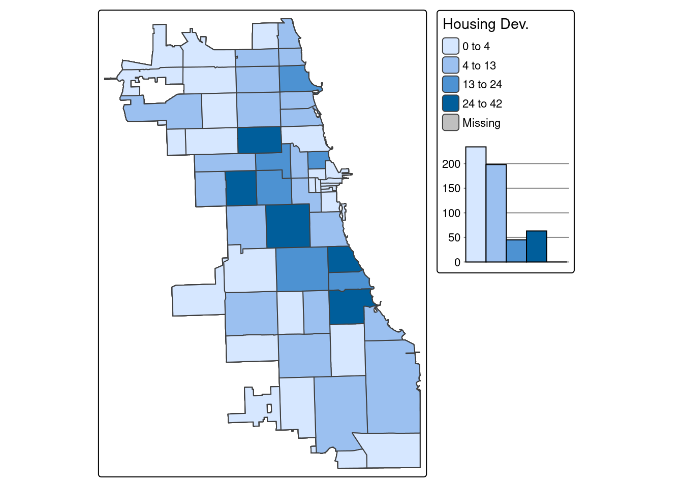

Note: You may get an error about missing the package ggplot2. To address this, just install that package and then rerun the command above.

install.packages("ggplot2")

Example 2. Number of COVID-19 Cases per Zip Code

Let’s do the same, but plut a different variable. Select a different variable name as your parameter in the ‘tm_fill’ parameter.

tm_shape(Chi_Zipsf.3435) + tm_polygons("Case.Rate...Cumulative",
              legend.hist = TRUE, style="jenks", 
              pal="BuPu", n=4, title = "COVID Case Rate") + 

  tm_layout(legend.outside = TRUE, legend.outside.position = "right")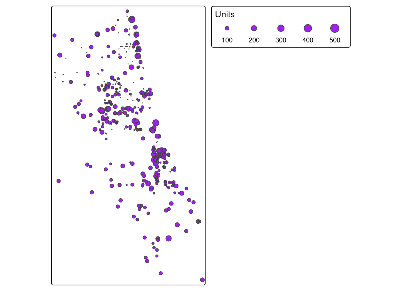

A.7.2 Map Overlay

Example 1. Affordable Housing Developments & Zip Code Boundaries

We previously translated the housing dataset from a CSV to a spatial object. Let’s take an attribute connect with each point, the total number of units per housing development, and visualize as a graduated symbology. Points with more units will be bigger, and not all places are weighted the same visually.

We use the “style” parameter to add a standard deviation data classification break. Check out tmap documentation for more options, like quantiles, natural jenks, or other options.

tm_shape(housing.3435) + tm_bubbles("Units", col = "purple", style = "sd") 

## 

## ── tmap v3 code detected ───────────────────────────────────────────────────────────────────────────────────────────────────

## [v3->v4] `tm_bubbles()`: instead of `style = "sd"`, use fill.scale = `tm_scale_intervals()`.
## ℹ Migrate the argument(s) 'style' to 'tm_scale_intervals(<HERE>)'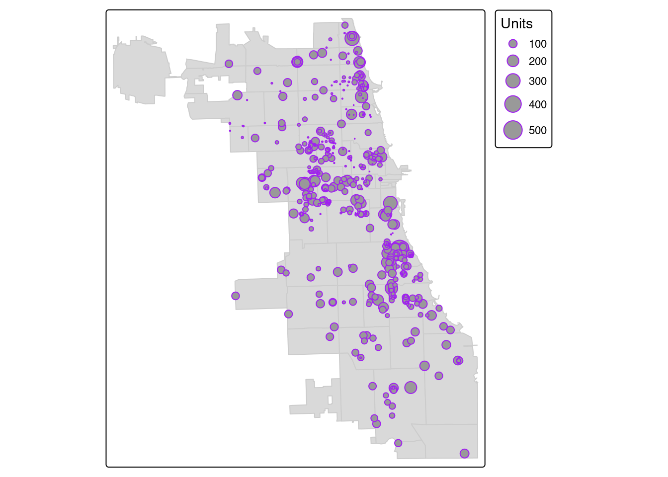

Then, let’s overlay that layer to the zip code boundary.

tm_shape(Chi_Zipsf.3435) + tm_polygons(col = "gray80") +
  
  tm_shape(housing.3435) + tm_bubbles("Units", col = "purple")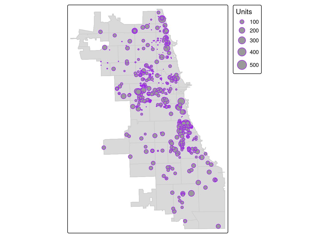 

You can also color-code according to the total number of units. Here, we’ll add a palette using a “viridis” color scheme, as a graduate color point map. For extra style, we’ll add labels to each zip code, update with a new basemap, and make the whole map interactive.

tmap_mode("view")

## ℹ tmap mode set to "view".

#Add Basemap
tm_basemap("Esri.WorldGrayCanvas") + 
  
  #Add First Layer, Style
  tm_shape(Chi_Zipsf.3435) +  tm_borders(col = "gray10") + 
    tm_text("zip", size = 0.7) +

  #Add Second Layer, Style
  tm_shape(housing.3435) + 
    tm_bubbles( col = "Units", style = "quantile", 
                pal = "viridis", size = 0.1) 

## 
## ── tmap v3 code detected ───────────────────────────────────────────────────────────────────────────────────────────────────
## [v3->v4] `tm_bubbles()`: instead of `style = "quantile"`, use fill.scale = `tm_scale_intervals()`.
## ℹ Migrate the argument(s) 'style' to 'tm_scale_intervals(<HERE>)'[tm_bubbles()] Argument `pal` unknown.

Example 2. COVID-19 & Methadone

In the first example, let create a map showing both COVID-19 and methadone clinic data (used in A.3). First, let’s add our zip code map.

With this overlay, we’ll add a “hack” to include the methadone clinic points in a legend.

tmap_mode("plot")

## ℹ tmap mode set to "plot".

##Add and style First Layer
tm_shape(Chi_Zipsf) + tm_polygons("Case.Rate...Cumulative", 
              style="jenks", pal="BuPu", n=4, title = "COVID Rt") + 
  
  ##Add Second Layer
  tm_shape(methadoneSf) + tm_dots(size = 0.2, col = "gray20") +
  
  ##"Hack" a manual symbology for dots in the legend
  tm_add_legend("symbol", col = "gray20", size = .2, labels = "Methadone MOUD") +
  
  ##Final Cartographic Styling
  tm_layout(legend.outside = TRUE, legend.outside.position = "right")

## 
## ── tmap v3 code detected ───────────────────────────────────────────────────────────────────────────────────────────────────
## [v3->v4] `tm_polygons()`: instead of `style = "jenks"`, use fill.scale = `tm_scale_intervals()`.
## ℹ Migrate the argument(s) 'style', 'n' to 'tm_scale_intervals(<HERE>)'[v3->v4] `tm_polygons()`: migrate the argument(s) related to the legend of the visual variable `fill` namely 'title' to
## 'fill.legend = tm_legend(<HERE>)'[tm_polygons()] Argument `pal` unknown.

A.8 Video Walkthrough

Here is a walkthrough of the module in video format. This presentation is provided by the author(s) of the module for your thorough understanding, so grab a cup of coffee and follow along:

Resources

For a deeper dive on topics discussed in this chapter, please check out the following. If you have a resource to add, feel free to suggest one by submitting an issue to our toolkit repository.

• For tips on using tmap, check out the online text, Elegant and informative maps with tmap by Tennekes and Nowosad.

• Try out more mapping with the ggplot2 library. The Maps chapter will give you a head start.

• We highly recommend Chapters 3-5 as mandatory reading in this classic, Geocomputation with R by Lovelace, Nowosad, and Muenchow. Perfecting selections and filters in the Attribute Data Operations chapter will help you become a data wrangling master. Perfect distance metrics and essential GIS operations in subsequent chapters.

• The Appendix in Gimond’s Intro to GIS online book has a super overview of R examples, not to be missed.

• Another superb resource is Analyzing US Census Data by Kyle Walker, with some of our favorite examples of extracing & reshaping data directly from the Census using code. Highly recommended!

---